Technical Report (Draft) – AI Playtesting

Introduction

If we train a reinforcement learning agent to play a card game, can we use it to playtest the game and provide important insights to game designer? This is the question that we are trying to answer. In the recent past, Reinforcement Learning has had a lot of success playing computer games. There are the popular examples of AlphaGo for Go and OpenAI for Dota2 where the AI agents have been highly successful at mastering the game. However, these were the result of a huge amount of human effort by researchers who were behind making reinforcement learning agents work and the seemingly unlimited computational resources at their disposal. Can this technique also be used by traditional game companies or even indie companies to develop something similar for their games? If yes, then having an AI playtester can help improve the time it takes to test a game design change.

In order to work on answering the question posed above, we started looking at games that have a deep strategy but still have a finite and discrete state and action spaces. Combat card games were a natural choice because they satisfy our requirements perfectly. Slay the Spire was the game we chose and settled on because of its deep strategy as well as simple and consistent rules.

After settling on Slay the Spire, we picked a single boss fight that we could work on. It was important to narrow the scope of our project because reinforcement learning is complex and it can become increasingly difficult if we try to create an agent that needs to do too many things at the same time. The boss that we picked is called ‘The Guardian’. This is a boss that multiple modes and forcing a boss into one mode or another can be crucial to avoiding heavy damage. Hence, there is a strategy to beating this boss effectively and it is something that the AI needs to learn in order to achieve a high win rate. As a result, it is good experimental setup to see if we can teach a reinforcement learning agent to identify this.

Overall System Design

There are three major components of the system we are trying to build. These are as follows:

Gameplay Kernel : This handles the gameplay logic and updates the game state depending on the progress of the game. The game state is available to the other components to use.
AI Module : This part is where the reinforcement learning agent is implemented. There are several helper classes that are used for communication with the other components of the system as well as some classes that are used for manipulating the training data.
Unity Front End : We use Unity to render graphics to display our game state. This front end system can also be used by human players to play the game. We have also created some custom tools that allow for interface with the AI Module and visualize the AI’s decision making mechanism.

First Steps

One of the first steps that we needed to do is to create our own copy of Slay the Spire in Python. We were planning to use Tensorflow and python to handle all of our reinforcement learning code. Having the game implemented in python would greatly improve the efficiency of the system and allow for ease of communication between the game system and the reinforcement learning module.

When we were done with the first iteration of the game, we had a version of the game that was playable through code.

Progress of the AI

Our current Reinforcement Learning agent is based on Deep Q-Learning. This a very popular reinforcement learning algorithms and has been used successfully in a variety of Reinforcement Learning problems.

The problem that we are trying to solve is difficult because the game is complex. Each card behaves differently and have mechanics that complement other cards. The sequence of playing cards makes a big impact on how much damage is done in a turn. The agent not only needs to learn the intricacies and strategies of the boss, it also needs to learn which cards to play and the correct sequence of playing them.

The number of possible states is very large. This is simply because there are a lot of different values that represent the current state of the game. Some of these include:

Player’s health
Player’s block
Boss’ health
Boss’ block
Damage for boss phase change
Player’s active buffs
Boss’ active buffs
Player energy level
Cards in hand
Cards in hand that are playable
Cards in the draw pile
Cards in the discard pile

The cards in the deck need to be predetermined. Although we have currently implemented 32 different cards, typically there are 10-12 cards in a deck at a time. There can be duplicate cards in the deck.

The action space consists of each card that can be played in the game. We break down a turn of the game into multiple steps. At each step, we feed into the neural network, the current state of the game. The output of the network are values that give the expected reward of playing a card. If we have 12 cards, the output would be a 12 length vector with each value indicating the expected reward of playing one card.

AI Strategies Tested

The following is a list of all the different AI strategies that we explored to make the Reinforcement Learning agent work.

Naïve Approach

The first thing we did was create a simple neural network that takes in all the game state parameters (mentioned above) as input and predicts the expected reward from playing each card. Here is a list of the different things we tried out under this approach.

Loss Function – Mean Squared Error (this has remained unchanged for all the subsequent experiments)
Reward Function – +1/-1 for win/loss
Activation Function – Relu for input and hidden layers. None for the output layer.

The problem that we ran in with naive approach was the expected q-values were spiraling out of control to become very large values (somewhere in the order of magnitude of 10^10). In fact, sometimes they were spiraling out of hand so much that they crossed the acceptable float limit in python and the program would just end.

In order to tackle this, we tried regularization (L1 and L2). This did help to swiftly cut down the problem but probably it went too far. Now the predicted q-values became too small. This was probably because the weights were becoming too big and in order to keep the growth of weights in check, the q-values also got affected.

The last important thing that we tried under the naive approach was then to change the activation functions for the input and hidden layers from relu to sigmoid. This worked well to prevent the exponential growth of q-values and also didnt make them too small. It was good to make the training work but the agent was not any good at actually playing the game.

One thing that is important to mention here is that with the above mentioned strategies, the agent was performing exactly as good as a random bot (a bot that plays random cards in each turn). Our theory, from observing the agent’s behavior is that the agent learned that one card (defend) is the best in any and all situations. Similarly, it had second, third, fourth best cards although these fluctuated more than the first.

Splitting Into Three Models

Desperate to make things work, the next thing we tried was a little unconventional. We split the entire state space into three parts and trained a model individually for each. Each of these models would predict a set of q-values that we would then weight equally to get the final set of q-values. Although assigning equal weight to each was arbitrary, the idea was to modify these weights if this approach showed any promised. These three subparts of the state space were:

Player and Boss Basics : This consisted of the simple player and boss information which include health, block values and buffs.
Cards : This consisted (only) of in-hand and playable cards. It also include player energy (since energy is closely linked to cards).
Boss Intent : This was the last piece which included the boss intent values.

The biggest criticism of this approach is of course that it breaks the Markov Assumption of every state only being dependent on the previous state. For example, the current boss intent state may have little to do with the previous boss intent state. This means that it become harder for the AI agent to learn how to play sequences of cards.

With that being said, this model showed surprising promise over the previous method. We got to a winrate of around 15% (although with a very easy game setting where the boss only had 100HP) which was higher than the random bot at 7-8%. What was even more interesting was that individually these three methods did not perform as good. The basic model had a winrate of ~8-10% on its own, the card model was very low at ~0.7-1% and the boss intent model was at ~8-10%. However, when these models were brought together, to our surprise, they performed significantly better.

The cards model doing exceptionally worse than its peers is understandable. Information about which card is in hand does not really give the AI any information about performing better. However, we would still expect the AI do to at least as good as a random bot by simply ignoring the state input information and turning the problem into a multi-armed bandit problem. This strategy could possibly be better than random bot as well because the agent is always playing the card which gives the best reward on average.

Reward Function Modifications

Till this point, we were trying to train the model by only giving it a +1 reward for winning or a -1 reward for losing. We figured that one reason for the agent not learning much could be that it needed a much higher number of iterations to train on before the methods mentioned above showed any significant results. Since we could not afford this luxury, we theorized that we could improve training by crafting a custom reward function that rewards achievements in intermediary states.

Crafting a reward function like this is difficult and it has the obvious limitation of the agent never going beyond the strategy being supported by the reward function. This method also has the risk of us communicating to the agent a little too much about what we think is the best way to win the game.

While we understood the risk, we were looking for ways to make the agent learn so we decided to give this a shot. To implement the reward function, we first needed to highlight some of the game state values on the basis of which a models decisions can be recorded.

The first and the easiest one to program was health. If the boss loses health, it is almost always a good thing. When the player loses health, it is almost always a bad thing. Hence, we added a small intermediary reward for the boss losing health and the player blocking boss damage to conserve health.

The next step was to reward buffs which are much more complicated. The benefit of playing a buff card can be felt after a few other cards have been played. To do this, we added a buffer that stores all the states of a game. At the end of the game, it looks back to see all the card plays where the player or boss gained buffs. Then it would look ahead and calculate the impact of playing a buff in terms of the damage it did. This damage value was then used to reward the card which created the buff.

Although implementing the above did take considerable effort, it did not really improve anything. We were exactly where we had started with the winrate being close to or lower than the random bot. Around the same time that we implemented this, we also decided to change the game setting to match what a real player sees. We increased the boss health to 240 and reduced the player health to 75. All of these changes made it so that the average win rate we were getting at this point was ~0.5%.

Handling End Turn Actions

Another thing we did around the same time as implementing the reward functions was to change the way we handled the end-turn actions.

In the real game of Slay the Spire, the player needs to explicitly choose when they want to end their turn. There is a button in the game for ending turn. Since this is a core part of the game loop and is an action made by the player, we had included a neuron/node in the action space for ending turns. Up until this point, this action was essentially treated the same as playing a card. This meant that there was a reward value associated for the action of ending turn which the agent had to learn over time.

The problem we noticed with the end turn action was that some times the agent started ending turns for absolutely no apparent reason. This was in ways that a human player would never do. One of the issues with attributing any sort of negative reward to cards, while keeping the end-turn action as neutral (no negative reward), was that the agent would get into a local optima of always ending turns.

The first way we thought of combating the problem of ending turns was to give the agent a reasonably high negative reward for playing choosing the ending turn action. This method has a glaring downside – the agent will not end the turn even it should, even if it no longer has any playable cards! It would simply keep trying to play unplayable cards and this would go on forever.

In order to combat this problem, we had to come up with a way of attributing a negative reward for ending turns as well as trying to play unplayable cards. There was no easy way to do this, but one of the things we tried was to make the negative reward of ending turns dependent on the player energy. So if the agent tries to end turn when there is still 1 or more energy left, we give it a negative reward proportional to the remaining energy. If there is no remaining energy, then there is no negative reward for ending the turn.

This sounded reasonable in theory but in practice it was still unstable. We also had to think about the negative reward for trying to play unplayable cards because it was important for the agent to learn that. This had to be a constant value and completely arbitrary.

In the end, we decided to completely remove the end-turn action. We modified the agent to keep playing actions until it has no playable cards left. Upon reaching the state where it has no playable cards, the turn automatically ends. Again, this change in isolation did not do much for immediately improving the win rate but it was surely responsible in a way for our moderate success yet to come.

Handling Unplayable Cards

In line with the handling of end-turn actions as discussed above, we were also thinking about how to handle playing unplayable cards. To that end, there were several approaches we considered.

The simplest approach was to have a selection mechanism that operates on the q-values predicted by the AI. So instead of forcing the AI to choose playable cards, we just select the card with highest q-value that is also playable. The disadvantage of doing this is that this process is invisible to the AI. From the perspective of the AI agent, the card it predicts to be the best may not often be the card that is played. Secondly, the AI may have an unfairly high q-value associated with playing a particular unplayable card, but because it can never be played, the AI will never learn to update the incorrect q-value. This means that the AI can be left thinking for long periods of time that an unplayable card will give the maximum reward when in fact, the card is unplayable and hence an illegal move.

The next approach was to negatively reward playing an unplayable card and return the AI to the same state as it was in when it chose the unplayable card. This meant that choosing an unplayable card would result in no state change but the agent would still get a negative reward. This seemed like a wise idea at the time but it did not really work out. This mechanism coupled with the negative reward for end-turn (as mentioned above) would often result in local optima and the agent would stay in the same state looping over and over again with playing unplayable cards. The thinking behind this was that after a certain number of looped states, the agent would drive down its high q-value predictions of unplayable cards and place a higher value for playable cards. However, in practice this never happened correctly. We even shifted from sampling batches from an experience buffer for training to simply just taking the most recent state-action-reward tuple and use it to train. Again, this did not really work out very well and we abandoned this idea.

The last approach we took (and stuck with) was to give a negative reward to the playing an unplayable card and end the game. What this effectively meant was that the agent would lose automatically if it tried to play an incorrect card and the negative reward for doing this was a little higher than losing from taking damage from the boss. The reason we had a higher damage for losing by playing the wrong card was to ensure that the agent does not purposefully try to end the game by playing an unplayable card when in fact it can still play for more turns but thinks victory is impossible. This strategy proved to be effective and we did see the agent training successfully. Within a few number of games (~1000) it would learn to not play unplayable cards. It would learn this quite well in fact, so much so that after around ~2000 games, it would rarely ever play unplayable cards anymore. This was great because it meant that at the very least, the agent has understood the difference between playable and unplayable cards. This left us to focus on teaching the agent other important things like card play sequence and blocking incoming damage.

Incremental Discounting Factor

Despite efforts to modify various parts of our experimental setup, nothing was really working out. The poor winrate that we got since we implemented the realistic player and boss health values (player 75HP and boss 240HP) had not really improved. We initially got something along the lines of ~0.5-1% and even with all of the other strategies we tried, we ended up with something along the lines of ~1-2%.

We curious about why things were not working so much so that the results were abysmal. One of the things we had been encountering multiple times since the start of the project was this situation where q-values would grow quickly to be very large numbers in the orders of magnitude of 10^10 and beyond. This was strange because the reward values that are being predicted here were nowhere close to being that large.

A theory we devised to explain this phenomenon was of the cyclical q-function. The temporal difference target that we use to come up with the target q-values uses the following equation:

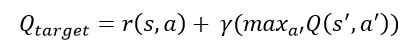
Here r(s,a) is the reward from taking action a in state s. Taking action a results in a state transition from s to s’. Action a’ is then chosen such that it is the maximum q-value of all possible actions in the new state s’. Gamma is the discounting factor used to discount future rewards and assign a higher importance to immediate reward.

This q-target value is then given to the network as being the target value it should predict for action a in state s. Thus the neural network must update its weights and biases so that the next time it encounters state s, it predicts a q-value for action a that is now closer to the value calculated by the above mentioned q-target.

However, if you notice here, the value of Q(s’, a’) is calculated by using the current model to predict the q-value for all possible actions for the new state of s’. This results in somewhat of a paradox. This is because the value of the q-target is used to update the weights and biases of the model. This in turn makes the q-target value itself incorrect since q-target depends heavily on the model’s prediction for state s’. Thus if we use the model updated using q-target to predict q-target again for the same state s, we would end up with a slightly different q-target value. The q-target value is hence non-stationary and led us to believe that it could be why the training was unstable.

In a quick attempt to resolve this, we made the gamma value zero. The negative implication of doing this is that the model then becomes extremely myopic, only worrying about the immediate reward and completely ignoring longer term rewards. However, we were curious to see if this would resolve our problem and prove our theory of the cyclical reward function. The result was that it did and the training results improved significantly. We went up to an ~8% winrate upon implementing this. Our model was training correctly and we could see it converging after many iterations. This was a ray of hope because we had being trying a lot of things that nothing seemed to be working and this did.

However, we knew that this was no victory. The agent cannot truly hope to be good at the game by simply beating the random bot which was at ~5-6%. The agent had to do much better and for this it had to account for longer term reward. To this end, we decided to implement 2 q-models. One of these model would be called q-predict and the other would be called q-train. The idea is to split the predicting and learning functionalities and make one model responsible for each. The motivation for doing this is to keep the q-target stationary, at least for a fixed number of iterations so that the learning model can correctly learn the q-values it needs to predict. The way the q-predict and q-train models work is shown below.

Initialize q-train to a model with random weights and q-predict to be null. Initialize gamma (discounting factor) to zero.
If gamma is zero, use q-train for making q-value predictions. Otherwise use q-predict for making q-value predictions.
For a fixed number of iterations: Train the q-train model using q-predict for making predictions (If gamma = 0, use q-train to make predictions).
Increment gamma by a arbitrary value.
Make q-predict = q-train.
Initialize q-train again with random weights.
Go back to step 2.

As you can see, as result of fixing the q-predict model and only updating it after a fixed number of iterations, we give time for the q-train model to learn on a stationary q-target. This method worked much better than keeping the gamma at 0 perpetually and improved our winrate to ~10%.

Choosing the value to increment q-value with is arbitrary. We chose 0.2 to be a good value but other values could also work, maybe some would even work better. The number of iterations after which we update gamma and the q-models is also arbitrary. We saw that keeping it at least around 100,000 worked well. While this can change and give better results, we found that if we make the number of iterations smaller, say 1000-10000, we start to see the same stability once again.

Action Masking

Another approach that we tried to prevent the agent from playing unplayable cards was to add a action masking layer when calculating q-targets. Since the game state contains information about which cards are playable, we can easily infer the unplayable cards. Since unplayable cards have a negative reward associated with them, we can directly assign a q-value to them during training that is equal to the negative reward of playing unplayable rewards.

This means that when we calculate the q-target vector for all possible cards, we replace values pertaining to unplayable cards to be equal to the negative reward of playable an unplayable card. If you remember from above, the negative reward of losing by playing an unplayable card is the highest. This means that unplayable cards cannot have a lower reward than the negative reward from playing unplayable cards.

This technique worked wonderfully and resulted in the agent learning very quickly which cards were unplayable. If earlier it took ~1000-2000 games for the agent to learn, with action making it took around ~200-300 games to learn this. This meant that the agent had more time to learn the correct actions.

With this technique implemented, we suddenly started getting a winrate of ~60%. This was a monumental increase in winrate however, it not only because of the last step. We believe that all the small improvements we made along the way to make our experimental setup better compounded and resulted in a very high increase all of a sudden. Similar to fixing the last piece in a big system and everything suddenly starts working correctly.

Moving Away from Reward Shaping

Before halves, we had achieved a breakthrough in the win rates by developing an elaborate win rate using an elaborate reward function. This was useful when we started using it because we were able to get a cheap rise in the win rate. However, it was sort of cheating in a sense because we as players of Slay the Spire already knew which cards were strong were weak. We also knew how each buff worked and how buffs could have impact beyond a single card turn. All of this information went into the reward shaping. For buffs, we tracked the damage that was done in subsequent turns to generate a reward value for the buffing card.

However, this came with its own set of challenges.

Buff Duplication: This of course got complicated when two cards played the same buff in succession such that the effect of the first card had not worn away yet. We worked around this problem by rewarding both cards the full reward amount of the buff. Of course, this could inflate the effect of buffs by artificially increasing their reward values.
Arbitrary Rewards: The problem with setting rewards like this is that the reward values can be very arbitrary. We get to decide how much should one card be rewarded compared to the other. Even if we try to standardize this by reward cards based on the damage they deal, it gets complicated when we think about buffs. In Slay the Spire, we even have the option of playing block cards which can reduce incoming damage. Here comes the question of how much should attack cards be prioritized over block cards. All of these questions were answered by setting arbitrary values. The idea was that we would adjust them if the method showed promised. If it worked out, we could always make these modifications later to improve the model. However, we found that balancing these arbitrary values is extremely hard and we would always feel like it is not correctly balanced. At the end, it started feeling like we were pushing the AI to favor one strategy over by the way of reward shaping.
Not generalizable and difficult to extend: One of the more obvious issues with this sort of reward shaping was that it is very difficult to extend. If new cards are introduced or new buffs are introduced, then we need to go back and add more code to the reward shaping functions. This makes the entire method very hard to generalize to new cards. And we definitely wanted to support the feature of allowing our users to create new cards.

In the end, we scraped the entire reward shaping idea and moved towards treating each card as equal and only being bothered by how much a card contributes to wins. This is much easier to do because essentially, cards or card combinations leading to wins are prioritized over cards that do not cause wins.

We started using a technique to calculate returns which is popularly known as Monte Carlo returns in the Reinforcement Learning literature. The way this works is by waiting till the end of the game and then looking at the reward obtained and the card sequence leading to this reward. Each card in the sequence gets a discounted reward based on how close or far it is from the end turn. Cards in the sequence that are close to end receive more reward since they are discounted less. Cards in the sequence that are farther from the end receive lesser rewards since they are discounted more. Once this reward calculation is done, all the state-action pairs of the entire game are collectively added to the replay buffer.

This method proved to be quite effective. It increased the win rate on the same test deck to around 80% which is the highest that we got. At this point it is important to mention that this jump in return is not only because of the Monte Carlo returns. There were a lot of minor optimizations that we did along the way that caused jumps in reward. However, the greatest jump and most impactful for our project was this particular one.

Reducing Model Complexity

The last challenge that needed to be overcome was reduction in model complexity. The real motivation to reduce the model complexity was that we were looking to package the entire playtesting process into an application which was meant to be user friendly to designers. Before we made the model complexity adjustments, training times could take anywhere from 24-36 hours. This was not only because of the model complexity but also because of the high number of iterations. Earlier, we were training the application for up to 50,000 iterations in the hopes that it would keep improving. Generally what we found was that models improved up until 20,000-25,000 iterations and plateaued after that point. However, since we were still in the experimentation phase, we were hopeful and trained for much longer.

This had to change when we were packaging the process into an application suitable for designers. 24-36 hours of training is unappealing and it was in our interest to try and bring it down. This involved getting rid of large neural networks containing 512 neurons per layer and 5 layers. We brought down the number of neurons in a layer from 512 to 128 for the first hidden layer, to 64 for the second hidden layer and to 32 for the third hidden layer. We also got rid of one layer completely. This was responsible for effectively culling the training time in half. Additionally we also decreased the recommended number of iterations to 15000. These changes added up and brought down the training time to 6-8 hours.

At this point you are probably wondering if reducing the model complexity caused a change in the AI’s performance. It did cause a minor drop in AI’s performance (about 5%) but only due to the lower number of iterations. Reducing the number of parameters in the model did not really cause a noticeable change at all reaffirming that big is not always better. We saw that by training the smaller network for more iterations resulted in very comparable performance.